The Checkerboard Metropolis Algorithm Explained.
Date created: July 28, 2023
Last Updated: August 19, 2023
In statistical physics, the Ising model assumes that the physical system of magnets can be mathematically represented by a lattice arrangement of molecules. In this model, every molecule possesses a "spin", which can align either upwards or downwards corresponding to the external magnetic field's direction. We will represent these spins +1 and -1 respectively as shown in the figure below (others represent the alignment as 0 and 1).
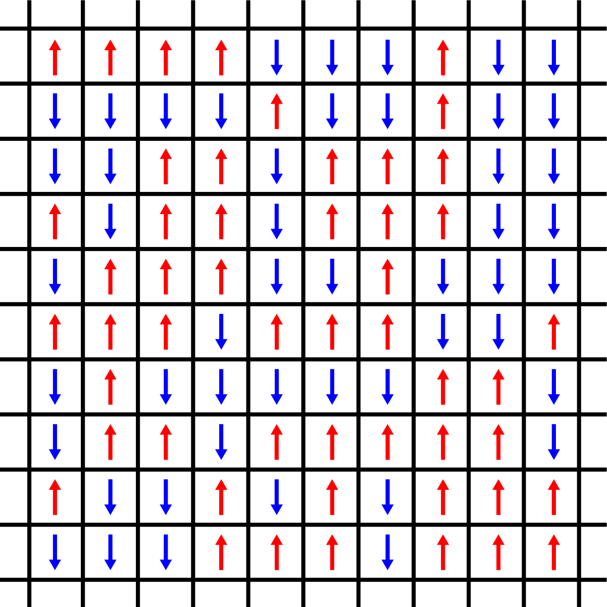
10x10 2D Ising model with random spins
Phase transition can be identified using the model as a simplified representation of reality. Phase transition often happens when the system moves from one zone to another and the temperature changes. The most common phase transition seen is between states of matter. For instance, from solid to liquid (ice to water). Similar to the phase changes in the states of matter, there is a phase transition in the Ising model as well. The model displays paramagnetic-ferromagnetic phase transition. Ernst Ising solved the 1D Ising model, although it did not indicate a phase transition at a positive temperature. Lars Onsager, on the other hand, was able to demonstrate phase transition \((T_c = 2.269)\) for the 2D Ising model.
One way to study the critical phenomena — the behavior of the system near a critical point where a phase transition occurs — of the Ising model is through Monte Carlo (MC) simulations. In a Monte Carlo simulation, instead of solving a problem analytically, random numbers are generated to simulate the behavior of a system or process. These random numbers are used as inputs to the mathematical model representing the problem, and the model's response is analyzed statistically.
A type of Monte Carlo Simulation is the Metropolis Algorithm. The pseudocode is as follows:
- Choose an initial state \(S(0)=(S_1,\ldots,S_N)\)
- Choose an \(i\) randomly or sequentially and calculate \(\Delta E=-2S_ih_i\)
- If \(\Delta E\geq 0\), then flip the spin, \(S_i \to -S_i\). If \(\Delta E < 0 \), draw a uniformly distributed random number \(r\in[0,1]\). If \(r < e^{\Delta E / k_B T}\), flip the spin, \(S_i\to-S_i\), otherwise take the old configuration into account once more.
- Iterate 2 and 3.
An implementation in Python is shown below:
######### MODULES #############
import numpy as np
import matplotlib.pyplot as plt
######### VARIABLES #############
lattice_n = 16 # number of rows
lattice_m = lattice_n # number of columns
seed = 1 # Set seed for consistency and reproducibility
temp = 0.5 # temperature (ferromagnetic)
eq_steps = 1000 # Equilibration steps
J=1 # Interaction constant
h=0 # External magnetic field
######### FUNCTIONS #############
def initial_state(N, M):
state = np.random.choice(np.array([-1,1]),size=(N,M))
return state
def mc_move(lattice, inv_T):
n = lattice.shape[0]
m = lattice.shape[1]
for i in range(n):
for j in range(m):
# Periodicity for neighbors out of index
ipp = (i + 1) if (i + 1) < n else 0
jpp = (j + 1) if (j + 1) < m else 0
inn = (i - 1) if (i - 1) >= 0 else (n - 1)
jnn = (j - 1) if (j - 1) >= 0 else (m - 1)
# Calculate neighbors
nb = lattice[ipp,j] + lattice[i,jpp] + lattice[inn,j] + lattice[i,jnn]
# Compute energy difference
spin = lattice[i, j]
deltaE = -2*spin*(J*nb + h)
if deltaE >= 0:
lattice[i, j] = -spin
elif np.random.rand() < np.exp(deltaE*inv_T):
lattice[i, j] = -spin
return lattice
def plot_ising(lattice, colorbar=True):
plt.imshow(lattice, cmap='gray', vmin=-1, vmax=1)
if colorbar == True:
plt.colorbar()
######### SIMULATION #############
np.random.seed(seed) # set seed for reproducibility
inv_T = 1/temp # Inverse temperature
lattice = initial_state(lattice_n, lattice_m) # Initialize the lattice
initial_lattice = lattice.copy() # Copy lattice for the plotting
# Equilibration
for i in range(eq_steps):
mc_move(lattice, inv_T)
# Plot the lattices
plot_ising(initial_lattice)
plt.show()
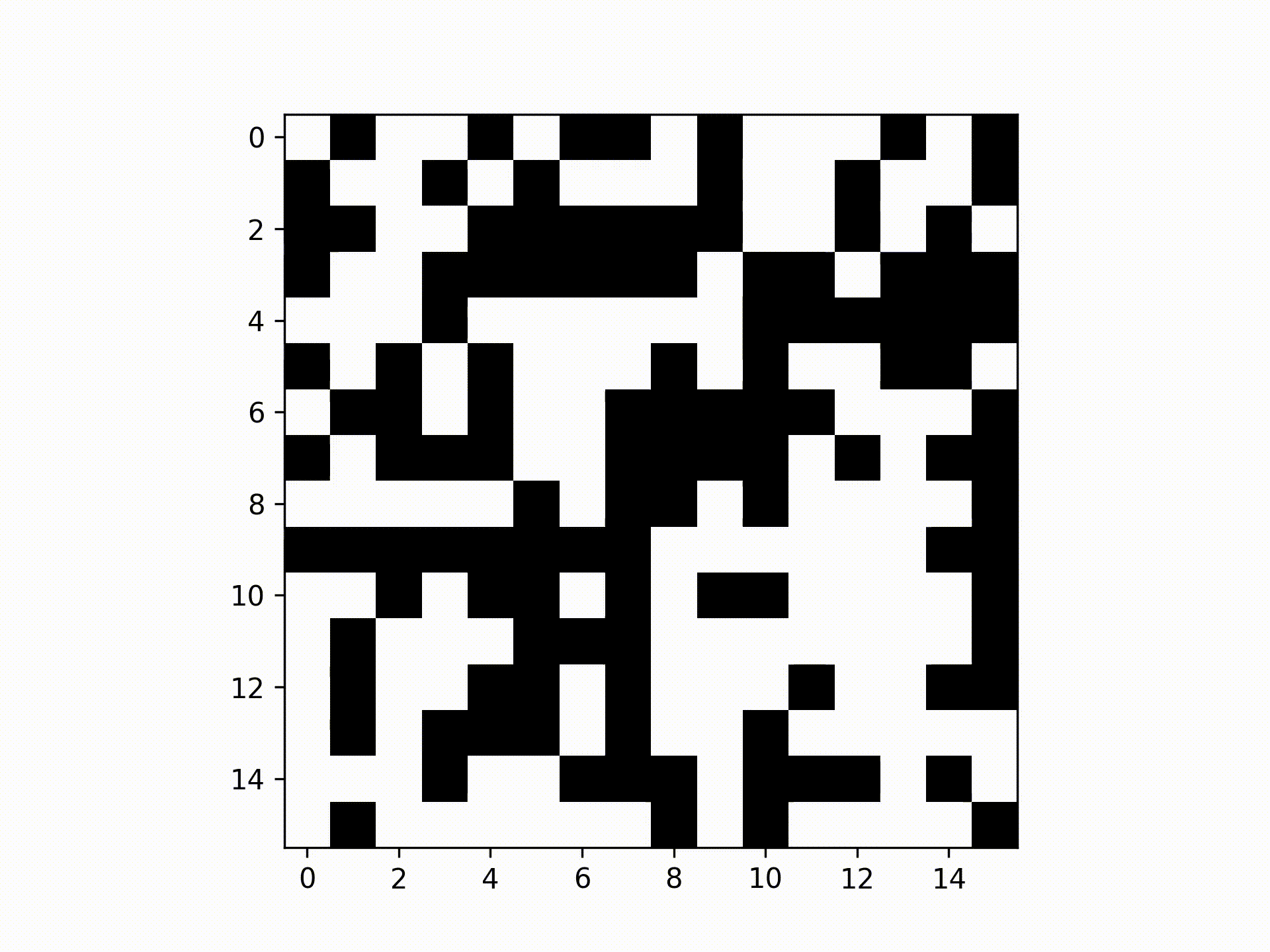
plot_ising(lattice)
plt.show()When we try to animate the flipping of the Metropolis simulation, it is shown below.
Metropolis Algorithm per update of spins.
The problem with the Metropolis algorithm is its performance — only a single spin is being flipped at a time. One way to strategize for the performance of the simulation is through parallel computing. Code can be run more quickly and efficiently with the aid of parallel computing. We could implement parallel computing using the multiple cores we have on our CPU. Although, a better option would be through the use of GPU as it allows faster computation.
To implement parallel computing, we must consider the dependency of each spin — the complexity of parallel computing remains a challenge for every application of it as it requires careful consideration of dependencies between tasks. If we’re going to update all of the spins at once, it would raise such problems:
- The neighboring spins for each iteration may differ, not allowing us to implement a random seed.
- The calculation of the properties of the model may have inconsistencies and fluctuations.
Thus, the checkerboard algorithm was created. It allows parallel spin updates exclusively within non-interacting domains. The pseudocode for the checkerboard algorithm is as follows:
- Populate an \(n\times m/2\) array of random values.
- Update spins on the lattice for the current color using the opposite-colored lattice spin values and the random value array.
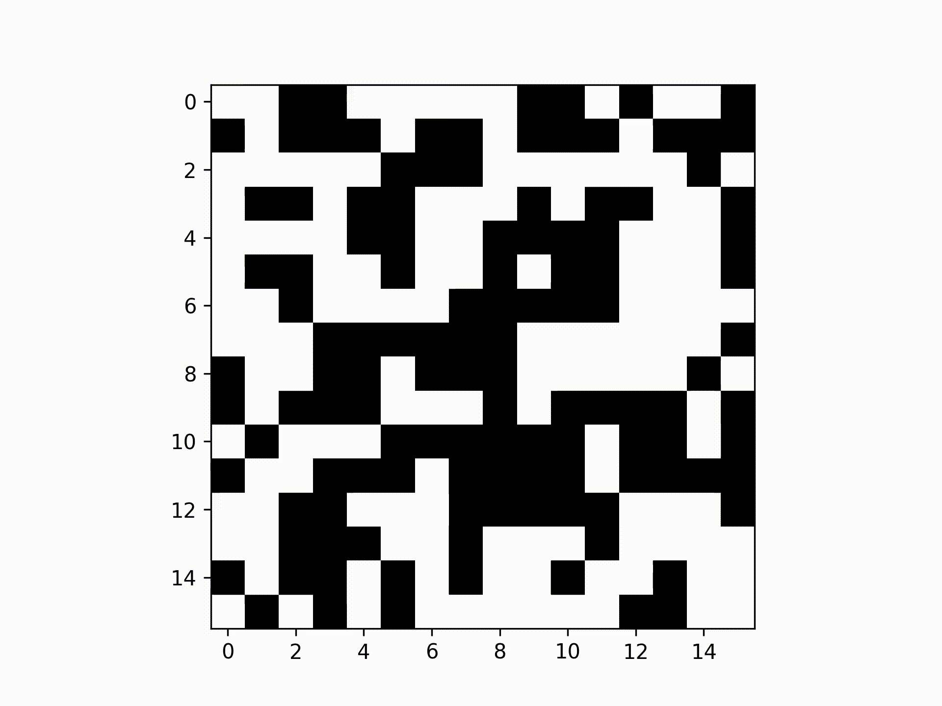
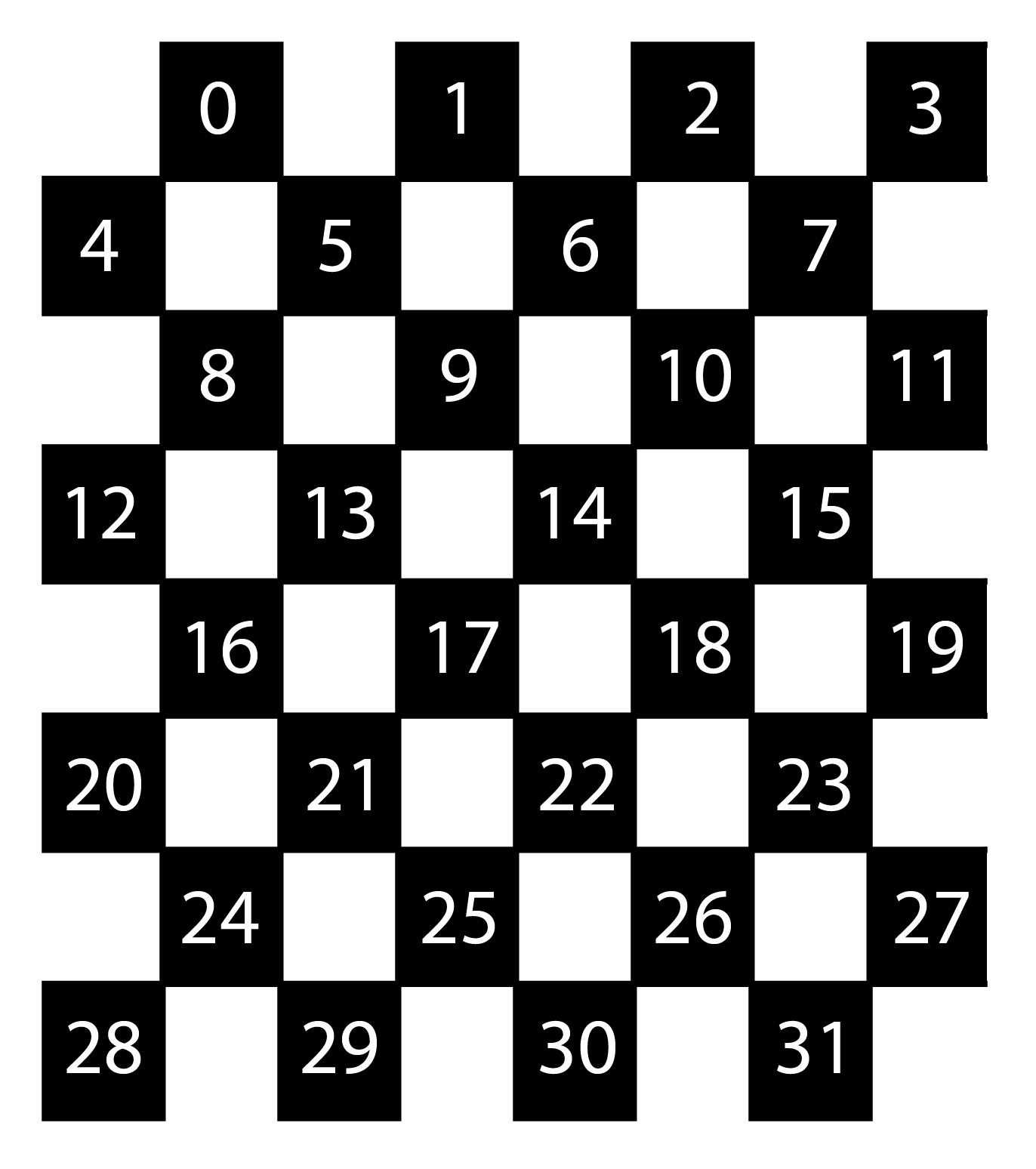
For the first step, an example of \(n\times m/2\) array is shown below. The image on the left is the array. When we convert it into the lattice, it would show the second image.
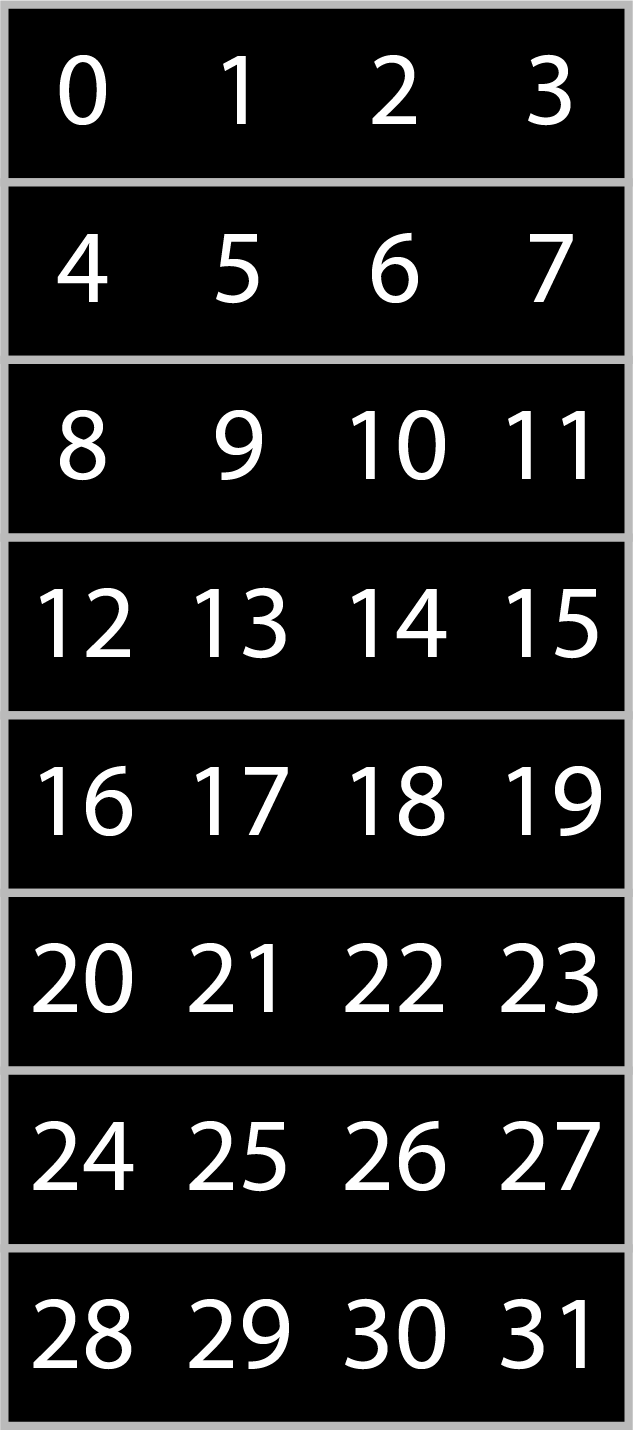
\(n\times m/2\) array (black lattice). The numbers correspond to the indices.
\(n\times m/2\) array when represented as a black lattice.
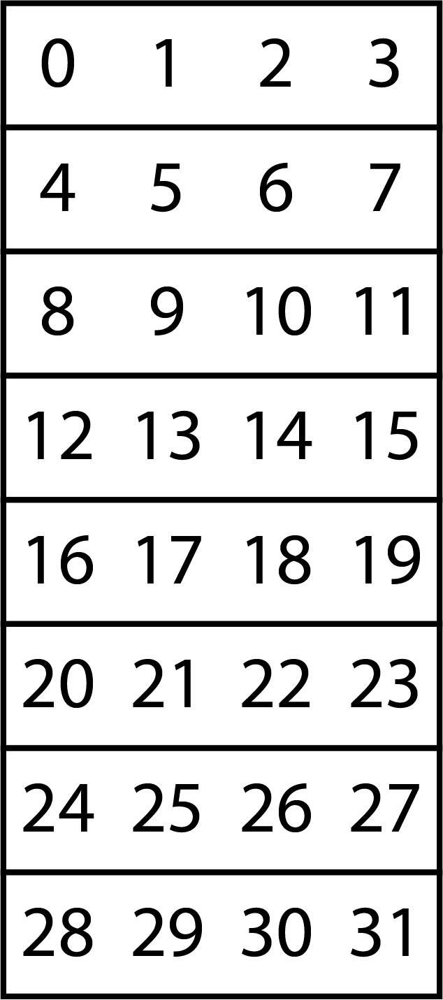
\(n\times m/2\) array (white lattice). The numbers correspond to the indices.
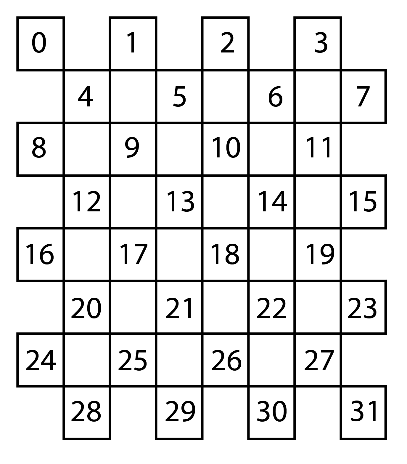
\(n\times m/2\) array when represented as a white lattice.
Combining the arrays would result in a checkerboard,

For the second step, we’ll update the following with the random values. From the images, the number only represents the indices. The images below show an array of random values. Similar to the metropolis algorithm, we’ll use the metropolis criterion. We’ll first calculate the $\Delta E$ of the spin. If \(\Delta E < 0\), we’ll use the Metropolis criterion \(r < e^{\Delta E/k_BT}\) using the random values we’ve generated.

We’ll do the update of the spins in parallel. The simulation of the checkerboard algorithm is shown below.
Checkerboard Algorithm per update of spins
The implementation using Python with the help of Numba to implement parallelization, we could run the following simulation.
######### MODULES #############
import numpy as np
import matplotlib.pyplot as plt
from numba import njit, prange
import time

######### VARIABLES #############
lattice_n = 512 # number of rows
lattice_m = lattice_n # number of columns
seed = 1 # Set seed for consistency and reproducibility
temp = 0.5 # temperature (ferromagnetic)
eq_steps = 1000 # Equilibration steps
J=1 # Interaction constant
h=0 # External magnetic field

######### FUNCTIONS #############
@njit
def set_seed():
	np.random.seed(seed)

@njit
def generate_lattice(N, M):
	return np.random.choice(np.array([-1,1], dtype=np.int8),size=(N,M))

@njit
def generate_array(N, M):
	return np.random.rand(N, M)

@njit(parallel=True)
def mc_move(lattice, op_lattice, randvals, is_black, inv_temp):
	n,m = lattice.shape
	for i in prange(n):
		for j in prange(m):
			# Set stencil indices with periodicity
			ipp = (i + 1) if (i + 1) < n else 0
			jpp = (j + 1) if (j + 1) < m else 0
			inn = (i - 1) if (i - 1) >= 0 else (n - 1)
			jnn = (j - 1) if (j - 1) >= 0 else (m - 1)

			# Select off-column index based on color and row index parity
			if (is_black):
				joff = jpp if (i % 2) else jnn
			else:
				joff = jnn if (i % 2) else jpp

			# Compute sum of nearest neighbor spins
			nn_sum = op_lattice[inn, j] + op_lattice[i, j] + op_lattice[ipp, j] + op_lattice[i, joff]

			# Compute sum of nearest neighbor spins (taking values from neighboring
			spin_i = lattice[i, j]
			deltaE = -2* spin_i*(J*nn_sum+h)
			if deltaE >= 0:
				lattice[i, j] = -spin_i
			elif randvals[i, j] < np.exp(deltaE*inv_temp):
				lattice[i, j] = -spin_i
	return lattice

@njit(parallel=True)
def combine_lattice(lattice_black, lattice_white):
	lattice = np.zeros((lattice_n, lattice_m), dtype=np.int8)
	for i in prange(lattice_n):
		for j in prange(lattice_m // 2):
			if (i % 2):
				lattice[i, 2*j+1] = lattice_black[i, j]
				lattice[i, 2*j] = lattice_white[i, j]
			else:
				lattice[i, 2*j] = lattice_black[i, j]
				lattice[i, 2*j+1] = lattice_white[i, j]
	return lattice

def plot_ising(lattice, colorbar=True):
	plt.imshow(lattice, cmap='gray', vmin=-1, vmax=1)
	if colorbar == True:
		plt.colorbar()

######### SIMULATION #############
set_seed() # set seed for reproducibility

lattice_black = generate_lattice(lattice_n, lattice_m//2) # m/2 array for black lattice
lattice_white = generate_lattice(lattice_n, lattice_m//2) # m/2 array for white lattice
initial_lattice = combine_lattice(lattice_black, lattice_white).copy() # get a snapshot of initial lattice

inv_temp = 1.0/temp # Inverse temperature

# Compilation
randvals = generate_array(lattice_n, lattice_m//2)
mc_move(lattice_black, lattice_white, randvals, True, inv_temp)

randvals = generate_array(lattice_n, lattice_m//2)
mc_move(lattice_white, lattice_black, randvals, False, inv_temp)

# Equilibration
start_time = time.time() # start timer for performance evaluation
for i in range(eq_steps):
	randvals = generate_array(lattice_n, lattice_m//2)
	mc_move(lattice_black, lattice_white, randvals, True, inv_temp)

	randvals = generate_array(lattice_n, lattice_m//2)
	mc_move(lattice_white, lattice_black, randvals, False, inv_temp)
end_time = time.time() # records end time
total_time = end_time - start_time

lattice = combine_lattice(lattice_black, lattice_white).copy() # combine black and white lattice
flips_per_ns = ((lattice_n * lattice_m * eq_steps) / total_time) * 1e-9
print('Finished simulation for the checkerboard algorithm...')
print(f'flips/ns: {flips_per_ns}')

# Plot the lattices
plot_ising(initial_lattice)
plt.show()
plot_ising(lattice)
plt.show()
Comparing the two simulations side by side, we could see its difference.

Metropolis algorithm per update of spins.
Checkerboard algorithm per update of spins.
The following results for low lattice sizes (figure shown below) are from our research paper, showing the benefits of parallel computing almost at all lattice sizes. Of course, there are still drawbacks to implementing parallel, but it only happens at a single lattice size and the difference isn’t that high.

Increasing the lattice sizes, we see substantial benefits of using the GPU.
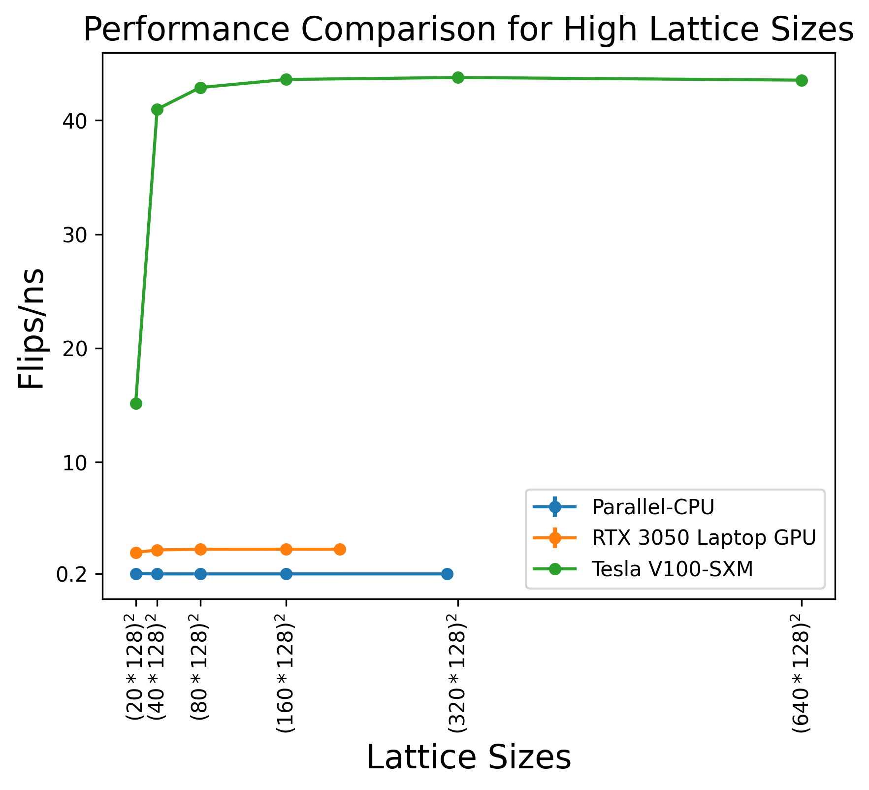
Tesla V100-SXM results are from Romero et al. (2020).
To conclude, accelerating the Monte Carlo simulation of the 2D Ising model enables more efficient exploration of the model's behavior, expands the range of system sizes that can be studied, and enhances the study of dynamic properties.
Note (Package Requirements)!!!
Please install the following packages for it to work:
- numpy
- matplotlib
- numba
References
[1] S. G. Brush, “History of the Lenz-Ising model,” Rev. Mod. Phys., vol. 39, no. 4, pp. 883–893, 1967, doi: 10.1103/RevModPhys.39.883.
[2] H. Gould and J. Tobochnik, Statistical and Thermal Physics: With Computer Applications. Princeton University Press, 2010.
[3] M. E. J. Newman and G. T. Barkema, Monte Carlo methods in statistical physics. Oxford University Press, 1999.
[4] N. Metropolis, A. W. Rosenbluth, M. N. Rosenbluth, A. H. Teller, and E. Teller, “Equation of state calculations by fast computing machines,” J. Chem. Phys., vol. 21, no. 6, pp. 1087–1092, Jun. 1953, doi: 10.1063/1.1699114.
[5] T. Preis, P. Virnau, W. Paul, and J. J. Schneider, “GPU accelerated Monte Carlo simulation of the 2D and 3D Ising model,” J. Comput. Phys., vol. 228, no. 12, pp. 4468–4477, 2009, doi: 10.1016/j.jcp.2009.03.018.
[6] K. A. G. Andal and R. C. Simon, “Parallel Monte Carlo simulation of the 2D Ising model using CPU and mobile GPU,” in Proceedings of the Samahang Pisika ng Pilipinas, 2023, p. SPP-2023-PA-06. [Online]. Available: https://proceedings.spp-online.org/article/view/SPP-2023-PA-06
[7] J. Romero, M. Bisson, M. Fatica, and M. Bernaschi, “High performance implementations of the 2D Ising model on GPUs,” Comput. Phys. Commun., vol. 256, p. 107473, 2020, doi: 10.1016/j.cpc.2020.107473.
[8] K. Binder and E. Luijten, “Monte Carlo tests of renormalization-group predictions for critical phenomena in Ising models,” Phys. Rep., vol. 344, no. 4, pp. 179–253, 2001, doi: 10.1016/S0370-1573(00)00127-7.